一、前言
二手车市场中,车辆价格受品牌、车龄、里程、马力、车况等众多因素影响,人工估价既依赖经验又容易产生偏差。如果能根据车辆的各项属性自动预测合理售价,无论是车商收车定价还是个人卖车参考,都有很高的实用价值——这就是典型的**回归预测问题**。
本文将基于一份包含 15 万条二手车交易记录的数据集,完整走一遍价格预测的建模流程:
+ 空格分隔的 CSV 文件读取方法
+ 混合类型特征的清洗:
object 列中的异常字符(如 -)处理+ 缺失值的差异化填充策略:分类特征填 -1、连续特征填中位数
+ 日期特征工程:从注册日期和上架日期计算**车龄**
+ 随机森林、LightGBM、XGBoost 三种树模型在回归任务上的表现对比
+ 特征重要性分析:为什么 LightGBM 更依赖业务特征,而随机森林/XGBoost 极度依赖单一脱敏特征
+ 错误样本分析:模型在哪些车上会严重低估价格
+ 测试集批量预测与结果导出
数据集包含 15 万条训练样本、5 万条测试样本,31 个特征,目标变量是二手车交易价格
price。* * *
二、数据探索
2.1 导入依赖与加载训练数据
import pandas as pd
import numpy as np
import matplotlib.pyplot as plt

# 设置中文显示
plt.rcParams['font.sans-serif'] = ['SimHei']
plt.rcParams['axes.unicode_minus'] = False

# 设置 DataFrame 表格打印显示格式
pd.set_option('display.max_columns', None)  # 设置最大显示列数:None代表全部列都显示
pd.set_option('display.width', 2000)        # 设置输出表格宽度,数值调大,单位字符
pd.set_option('display.max_colwidth', 30)   # 每列最大字符长度
""" 加载训练数据 """
train = pd.read_csv("8.used_car_train.csv", sep=r"\s+")  # 数据间使用的是空格来分隔
print(train.shape)
print(train.columns.tolist())
train.info()
 (150000, 31)
['SaleID', 'name', 'regDate', 'model', 'brand', 'bodyType', 'fuelType', 'gearbox', 'power', 'kilometer', 'notRepairedDamage', 'regionCode', 'seller', 'offerType', 'creatDate', 'price', 'v_0', 'v_1', 'v_2', 'v_3', 'v_4', 'v_5', 'v_6', 'v_7', 'v_8', 'v_9', 'v_10', 'v_11', 'v_12', 'v_13', 'v_14']
<class 'pandas.core.frame.DataFrame'>
RangeIndex: 150000 entries, 0 to 149999
Data columns (total 31 columns):
 #   Column             Non-Null Count   Dtype
---  ------             --------------   -----
 0   SaleID             150000 non-null  int64
 1   name               150000 non-null  int64
 2   regDate            150000 non-null  int64
 3   model              150000 non-null  float64
 4   brand              150000 non-null  float64
 5   bodyType           150000 non-null  float64
 6   fuelType           150000 non-null  float64
 7   gearbox            150000 non-null  object
 8   power              150000 non-null  object
 9   kilometer          150000 non-null  object
 10  notRepairedDamage  150000 non-null  object
 11  regionCode         150000 non-null  int64
 12  seller             150000 non-null  int64
 13  offerType          150000 non-null  float64
 14  creatDate          150000 non-null  float64
 15  price              150000 non-null  float64
 16  v_0                150000 non-null  float64
 17  v_1                150000 non-null  float64
 18  v_2                150000 non-null  float64
 19  v_3                150000 non-null  float64
 20  v_4                150000 non-null  float64
 21  v_5                150000 non-null  float64
 22  v_6                150000 non-null  float64
 23  v_7                150000 non-null  float64
 24  v_8                150000 non-null  float64
 25  v_9                150000 non-null  float64
 26  v_10               150000 non-null  float64
 27  v_11               150000 non-null  float64
 28  v_12               148531 non-null  float64
 29  v_13               146417 non-null  float64
 30  v_14               135884 non-null  float64
dtypes: float64(22), int64(5), object(4)
memory usage: 35.5+ MB
训练集共 15 万条、31 列。注意几个关键点:
+ 文件用**空格分隔**,读取时需要指定
sep=r"\s+";+
gearbox、power、kilometer、notRepairedDamage 四列是 object 类型,理论上应该是数值,说明里面混有异常字符;+
v_12、v_13、v_14 三个脱敏特征存在缺失值。2.2 特征说明
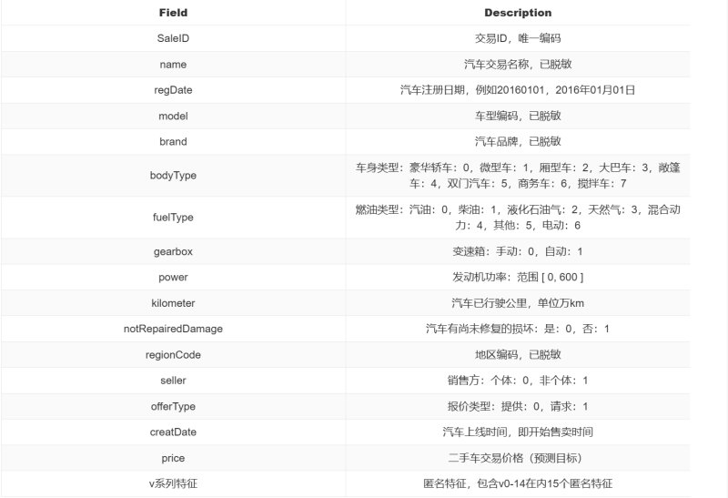
特征分为几类:基础信息(SaleID、name)、日期(regDate 注册日期、creatDate 上架日期)、车辆属性(model、brand、bodyType、fuelType、gearbox、power、kilometer)、车况(notRepairedDamage)、地区(regionCode)、交易属性(seller、offerType)、目标变量(price),以及 15 个脱敏匿名特征 v\_0 ~ v\_14。
* * *
三、数据清洗与特征工程
3.1 处理 notRepairedDamage 异常字符
打开 CSV 发现
notRepairedDamage 列的值中有字符 -,需要先转成数值。
print(train['notRepairedDamage'].unique())
train['notRepairedDamage'] = pd.to_numeric(train['notRepairedDamage'], errors='coerce')
print(train['notRepairedDamage'].unique())
['0.0' '-' '1.0' ... '1882' '7753' '2159']
[0.000e+00       nan 1.000e+00 ... 1.882e+03 7.753e+03 2.159e+03]
pd.to_numeric(errors='coerce') 会把无法转换的 - 变成 NaN,后续统一填充。3.2 缺失值统计与填充
""" 查看缺失值 """
missing_stats = train.isna().sum()
missing_percent = train.isna().sum() / len(train)
missing_df = pd.DataFrame({"缺失数量": missing_stats, "缺失占比": missing_percent})
print(missing_df[missing_df["缺失数量"] > 0])
                        缺失数量      缺失占比
notRepairedDamage  17558  0.117053
v_12                1469  0.009793
v_13                3583  0.023887
v_14               14116  0.094107
四个特征有缺失,采用差异化填充策略:
""" 处理缺失值 """
# 1. notRepairedDamage:把 '-' 替换成 NaN(前面已经做过了),再填充 -1 代表未知
train['notRepairedDamage'] = train['notRepairedDamage'].fillna(-1)

# 2. v_12、v_13、v_14:连续特征,统一用中位数填充(抗异常值)
for col in ['v_12', 'v_13', 'v_14']:
    train[col] = train[col].fillna(train[col].median())

# 3. 验证:确认没有任何缺失了
print(train.isna().sum().sum())
0
+
notRepairedDamage 是分类特征(0=无损伤、1=有损伤),用 **\-1** 填充表示"未知",与已有类别区分开;+
v_12、v_13、v_14 是连续数值特征,用**中位数**填充,比均值更能抵抗异常值的影响。3.3 类型转换
gearbox、power、kilometer 三列也是 object 类型,转为数值。
""" 类型转换 """
objectToInt = ['gearbox', 'power', 'kilometer']
for feature in objectToInt:
    train[feature] = pd.to_numeric(train[feature], errors='coerce')

print(train[objectToInt].dtypes)
print(train[objectToInt].isna().sum())  # 看 power/kilometer 有没有转失败产生NaN
gearbox      float64
power        float64
kilometer    float64
dtype: object
gearbox      1387
power        1188
kilometer    4191
dtype: int64
转换后产生了新的 NaN,继续填充:
""" 填充缺失值 """
train['gearbox'] = train['gearbox'].fillna(-1)
train['power'] = train['power'].fillna(train['power'].median())
train['kilometer'] = train['kilometer'].fillna(train['kilometer'].median())

# 再次校验缺失
print(train.isna().sum().sum())
0
+
gearbox(变速箱)是分类特征,填 -1 表示未知;+
power(马力)、kilometer(里程)是连续特征,填中位数。3.4 日期特征工程:计算车龄
regDate(注册日期)和 creatDate(上架日期)都是 YYYYMMDD 格式的整数,直接用没有意义。两者相减可以得到**车龄**——这是二手车定价中最核心的业务特征之一。
""" 处理两个日期特征 """
from datetime import datetime

def parse_date_safe(num):
    try:
        s = str(int(num))
        return datetime.strptime(s, "%Y%m%d")
    except:
        return np.nan  # 非法日期直接返回空

# 生成日期
train['reg_datetime'] = train['regDate'].apply(parse_date_safe)
train['create_datetime'] = train['creatDate'].apply(parse_date_safe)

# 计算车龄(年),存在 NaN 的地方车龄自动为 NaN
train['car_age'] = (train['create_datetime'] - train['reg_datetime']).dt.days / 365

# 查看有多少条非法日期样本
print("regDate非法日期数量:", train['reg_datetime'].isna().sum())
print("creatDate非法日期数量:", train['create_datetime'].isna().sum())
print("car_age缺失数量:", train['car_age'].isna().sum())
regDate非法日期数量: 11347
creatDate非法日期数量: 14116
car_age缺失数量: 20290
数据中存在不少非法日期(如月份为 00),用 try-except 安全解析,解析失败返回 NaN。车龄缺失的用中位数填充,然后删除原始日期字段。
""" 处理缺失值 """
train['car_age'] = train['car_age'].fillna(train['car_age'].median())

# 删除原始日期字段,不再使用
train = train.drop(['regDate', 'creatDate', 'reg_datetime', 'create_datetime'], axis=1)

# 校验
print(train['car_age'].isna().sum())
0
3.5 删除无用特征
SaleID 是唯一标识、name 是车辆名称编码,对价格预测没有实际意义,删除。
""" 去掉无用的特征 """
train = train.drop(columns=['SaleID', 'name'])
* * *
四、数据集划分
""" 划分 """
from sklearn.model_selection import train_test_split

X = train.drop('price', axis=1)
y = train['price']

X_train, X_val, y_train, y_val = train_test_split(
    X, y, test_size=0.2, random_state=42
)

print("训练集特征形状:", X_train.shape)
print("验证集特征形状:", X_val.shape)
训练集特征形状: (120000, 27)
验证集特征形状: (30000, 27)
按 8:2 划分训练集和验证集,最终特征维度为 27。
* * *
五、随机森林回归
5.1 模型训练与评估
""" 随机森林 """
from sklearn.ensemble import RandomForestRegressor
from sklearn.metrics import mean_squared_error, mean_absolute_error, r2_score

rf = RandomForestRegressor(
    n_estimators=100,
    max_depth=15,
    random_state=42,
    n_jobs=-1
)

rf.fit(X_train, y_train)
y_pred_rf = rf.predict(X_val)

rmse_rf = np.sqrt(mean_squared_error(y_val, y_pred_rf))
mae_rf = mean_absolute_error(y_val, y_pred_rf)
r2_rf = r2_score(y_val, y_pred_rf)

print("===== 随机森林回归评估结果 =====")
print(f"RMSE: {rmse_rf:.2f}")
print(f"MAE:  {mae_rf:.2f}")
print(f"R²:   {r2_rf:.4f}")
===== 随机森林回归评估结果 =====
RMSE: 1435.07
MAE:  632.41
R²:   0.9622
效果很好:
+ **R² = 0.9622**:模型可以解释 96.22% 的二手车价格波动;
+ **MAE = 632.41**:平均预测价格和真实价格相差约 632 元;
+ **RMSE = 1435.07**:对个别预测偏差很大的样本惩罚更强,最大误差会更高。
5.2 特征重要性
""" 随机森林特征重要性 """
feature_importance = pd.Series(
    rf.feature_importances_,
    index=X_train.columns
).sort_values(ascending=False)

plt.figure(figsize=(10, 6))
feature_importance.head(15).plot(kind='barh')
plt.title("随机森林 Top15 特征重要性")
plt.xlabel("特征重要性")
plt.gca().invert_yaxis()
plt.show()
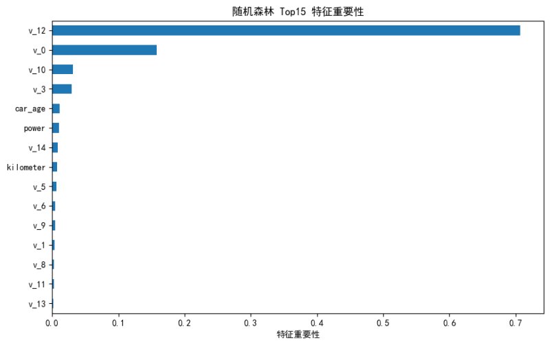
随机森林的特征重要性呈现出一个极端现象:**脱敏特征
v_12 占比超过 70%**,单一特征主导了整个模型,而业务特征(car\_age、power 等)权重很低。5.3 预测结果散点图
""" 随机森林预测结果 """
plt.figure(figsize=(8, 8))
plt.scatter(y_val, y_pred_rf, alpha=0.3, s=5)

# 理想预测线:真实 = 预测
plt.plot([y_val.min(), y_val.max()], [y_val.min(), y_val.max()], 'r--')
plt.xlabel("真实价格")
plt.ylabel("预测价格")
plt.title("随机森林:真实价格 vs 预测价格")
plt.show()
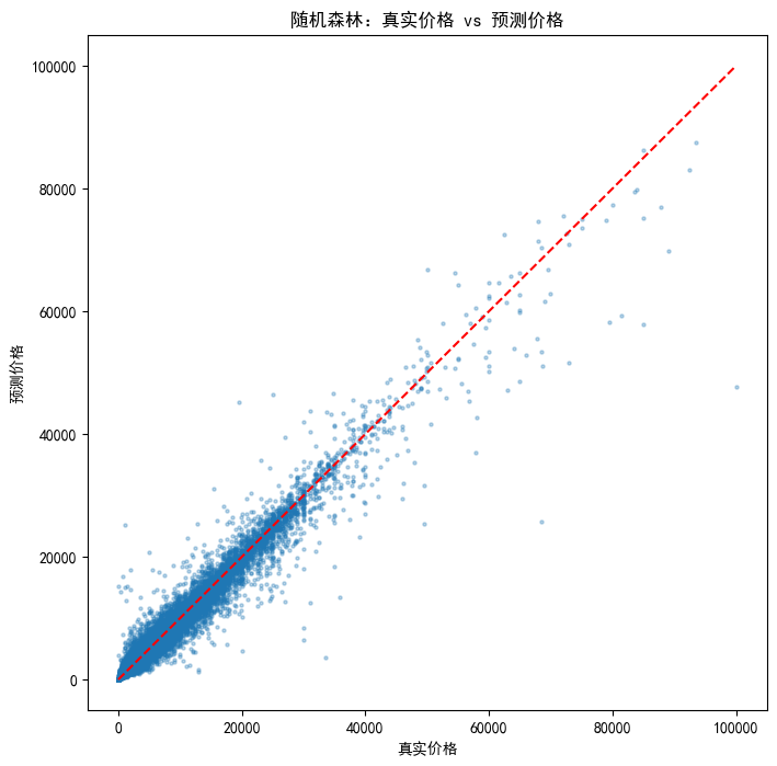
**散点图结果解读**:
+ **低价区间(0~40000)**:样本大量聚集,点紧紧贴住红色虚线,预测效果很好;
+ **高价区间(>40000)**:样本变少,点开始散开,**模型倾向于低估高价二手车**,很多真实高价车的预测价格明显低于真实值。
* * *
六、LightGBM 回归
6.1 模型训练与评估
""" LightGBM """
import lightgbm as lgb

lgb = lgb.LGBMRegressor(
    n_estimators=100,
    max_depth=15,
    random_state=42,
    n_jobs=-1
)

lgb.fit(X_train, y_train)
y_pred_lgb = lgb.predict(X_val)

rmse_lgb = np.sqrt(mean_squared_error(y_val, y_pred_lgb))
mae_lgb = mean_absolute_error(y_val, y_pred_lgb)
r2_lgb = r2_score(y_val, y_pred_lgb)

print("==== LightGBM 评估结果 ====")
print(f"RMSE: {rmse_lgb:.2f}")
print(f"MAE:  {mae_lgb:.2f}")
print(f"R²:   {r2_lgb:.4f}")
==== LightGBM 评估结果 ====
RMSE: 1374.24
MAE:  668.21
R²:   0.9653
LightGBM 的 R²(0.9653)和 RMSE(1374.24)都优于随机森林,整体预测误差更小。
6.2 特征重要性
""" LightGBM 特征重要性 """
feature_importance = pd.Series(
    lgb.feature_importances_,
    index=X_train.columns
).sort_values(ascending=False)

plt.figure(figsize=(10, 6))
feature_importance.head(15).plot(kind='barh')
plt.title("LightGBM Top15 特征重要性")
plt.xlabel("特征重要性")
plt.gca().invert_yaxis()
plt.show()
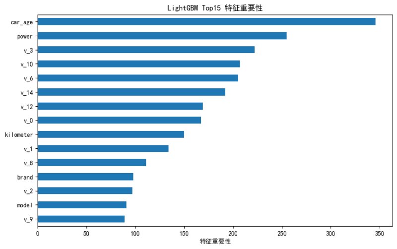
与随机森林形成鲜明对比:LightGBM 中 **
car_age(车龄)成为最重要特征**,其次是 power(马力),脱敏 v 系列特征的权重被分散开来,更符合二手车定价的业务常识。6.3 预测结果散点图
""" LightGBM 预测结果 """
plt.figure(figsize=(8, 8))
plt.scatter(y_val, y_pred_lgb, alpha=0.3, s=5)

# 理想预测线:真实 = 预测
plt.plot([y_val.min(), y_val.max()], [y_val.min(), y_val.max()], 'r--')
plt.xlabel("真实价格")
plt.ylabel("预测价格")
plt.title("LightGBM:真实价格 vs 预测价格")
plt.show()
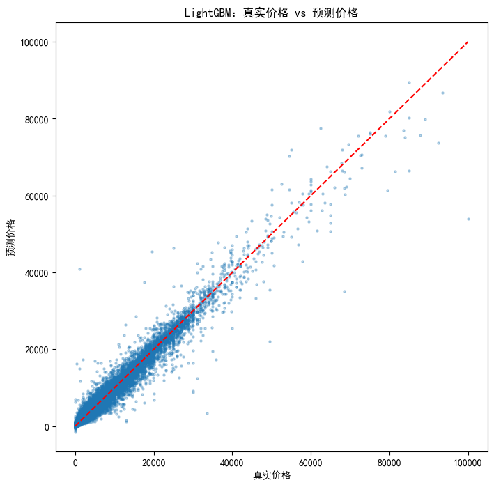
**指标解读**:
1. LightGBM 的 R² 更高、RMSE 更小,整体预测误差更小,总体性能优于随机森林;
2. MAE 略高于随机森林:说明 LightGBM 对**大部分普通样本**的平均误差稍大,但对少数大偏差样本(高价车)的抑制更好(RMSE 更低);
3. 两张散点图对比:LightGBM 高价区域的离散程度相比随机森林有轻微改善,但依然存在高价车低估的现象。
6.4 错误样本分析
把 LightGBM 预测偏差最大的样本捞出来,看看模型在哪些车上会严重低估。
""" LightGBM 错误样本分析 """
res_df = X_val.copy()
res_df["price_true"] = y_val
res_df["price_pred"] = y_pred_lgb
res_df["error"] = res_df["price_true"] - res_df["price_pred"]

# 真实价格高,预测偏低:误差>0,取前20个低估最严重样本
under_pred = res_df.sort_values("error", ascending=False).head(20)
print("===== 被严重低估的二手车样本 =====")
print(under_pred[["price_true", "price_pred", "error", "car_age", "power", "kilometer"]])
===== 被严重低估的二手车样本 ====="
        price_true    price_pred         error    car_age  power  kilometer
88326      99999.0  53949.851115  46049.148885  14.520548  114.0       15.0
112783     68530.0  35041.134055  33488.865945  16.747945  190.0       15.0
19083      33500.0   3353.919762  30146.080238   9.810959  150.0       15.0
55055      49500.0  21959.278278  27540.721722   3.493151    0.0        4.0
105451     30000.0   8773.564495  21226.435505  19.600000    0.0        6.0
22961      29900.0   9256.377785  20643.622215  19.715068  136.0        4.0
105007     92500.0  73702.229057  18797.770943   1.432877  600.0        1.0
112708     35840.0  17287.860623  18552.139377  19.019178  286.0       15.0
90978      31000.0  12453.386524  18546.613476  19.068493  231.0       15.0
132753     85000.0  66546.068309  18453.931691  21.731507  272.0        6.0
120445     79500.0  61417.724745  18082.275255  11.706849  360.0       12.5
10641      35000.0  19433.254230  15566.745770   3.356164  140.0        4.0
61532      81500.0  66362.201950  15137.798050   1.997260  495.0        2.0
46744      57900.0  42803.515394  15096.484606   1.057534  204.0        1.0
132361     40000.0  25518.765231  14481.234769  11.991781  340.0       15.0
3559       64999.0  50611.878146  14387.121854   3.205479  245.0        6.0
84400      49500.0  35423.860524  14076.139476   7.906849  420.0        7.0
10693      26500.0  12680.847029  13819.152971   5.991781  271.0        4.0
128940     30000.0  16505.980090  13494.019910  23.684932  326.0       15.0
5980       20000.0   6767.677339  13232.322661   8.498630  155.0       12.5
**低估样本分析总结**:
观察这批误差最大的样本,可以提炼出几个共性:
1. **车龄很大但价格依然很高的车**:比如车龄 1423 年,真实售价还能到 3 万10 万。正常规律是车龄越大价格越低,但这批属于特殊车型(经典老车、收藏车),脱离普通二手车的价格规律。训练集中这类样本数量极少,模型没有学到这种特例,所以严重低估。
2. **部分样本 power=0**:马力字段缺失(填了中位数但实际为 0),丢失了关键信息,模型无法识别高性能车辆,造成低估。
3. **低里程、大马力的高价新车**:车龄很小、里程很低、马力极高,属于高端车,样本量偏少,模型对高价区间拟合不足。
* * *
七、XGBoost 回归
7.1 模型训练与评估
""" XGBoost """
from xgboost import XGBRegressor

xgb = XGBRegressor(
    n_estimators=100,
    max_depth=15,
    random_state=42,
    n_jobs=-1
)

xgb.fit(X_train, y_train)
y_pred_xgb = xgb.predict(X_val)

rmse_xgb = np.sqrt(mean_squared_error(y_val, y_pred_xgb))
mae_xgb = mean_absolute_error(y_val, y_pred_xgb)
r2_xgb = r2_score(y_val, y_pred_xgb)

print("===== XGBoost 评估结果 =====")
print(f"RMSE: {rmse_xgb:.2f}")
print(f"MAE:  {mae_xgb:.2f}")
print(f"R²:   {r2_xgb:.4f}")
===== XGBoost 评估结果 =====
RMSE: 1462.61
MAE:  602.06
R²:   0.9607
7.2 特征重要性
""" 查看特征重要性 """
feature_importance = pd.Series(
    xgb.feature_importances_,
    index=X_train.columns
).sort_values(ascending=False)

plt.figure(figsize=(8, 6))
feature_importance.head(10).plot(kind="barh")
plt.title("XGBoost T10 特征重要性")
plt.xlabel("特征重要性")
plt.gca().invert_yaxis()
plt.show()
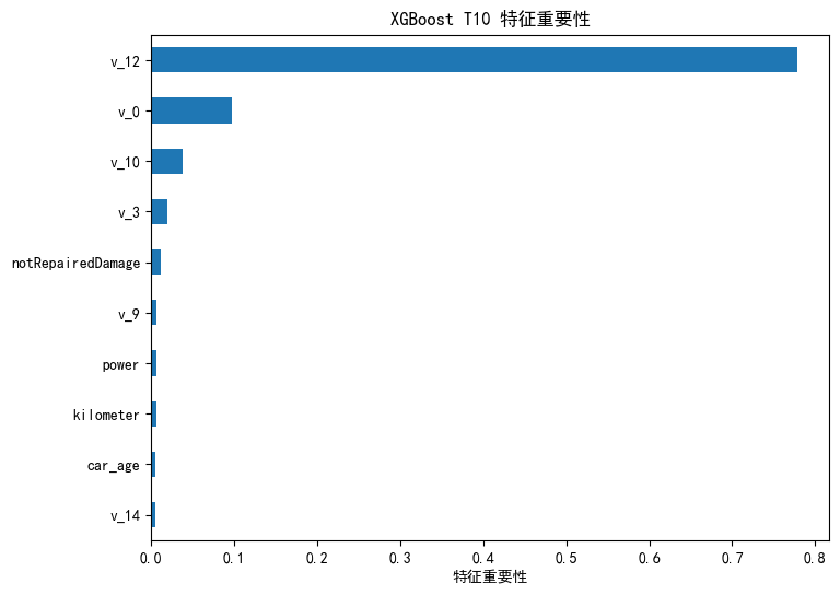
XGBoost 的特征重要性与随机森林类似:
v_12 权重接近 0.8,占据绝对主导,业务特征 car\_age、power、kilometer 权重极低。* * *
八、三模型对比
| 模型 | RMSE | MAE | R² | 特征重要性特点 |
| --- | --- | --- | --- | --- |
| 随机森林 | 1435.07 | 632.41 | 0.9622 | 高度依赖
v_12,单特征权重 70%+ || LightGBM | 1374.24 | 668.21 | 0.9653 | 业务特征
car_age、power 权重最高,特征分配均衡 || XGBoost | 1462.61 | 602.06 | 0.9607 | 同样极度依赖脱敏特征
v_12,和随机森林特征偏好很像 |**指标解读**:
1. **R²**:LightGBM > 随机森林 > XGBoost,LightGBM 对价格整体方差解释能力最强;
2. **RMSE**:LightGBM 最小,代表对**大误差样本**控制最好;XGBoost RMSE 最差,说明少数极端样本预测偏差更大;
3. **MAE**:XGBoost 最低,代表**绝大多数普通样本**的平均预测误差最小。
**总结**:XGBoost 在大部分常规二手车样本上预测更准,但遇到高价/特殊长尾样本时更容易出现巨大偏差;LightGBM 综合稳定性最好,且特征重要性更符合业务逻辑,因此选择 LightGBM 作为最终模型。
* * *
九、测试集预测
9.1 加载测试集
""" 预测集 """
test = pd.read_csv("8.used_car_test.csv", sep=r"\s+")
print(test.shape)
print(test.columns.tolist())
print(test.info())
(50000, 30)
['SaleID', 'name', 'regDate', 'model', 'brand', 'bodyType', 'fuelType', 'gearbox', 'power', 'kilometer', 'notRepairedDamage', 'regionCode', 'seller', 'offerType', 'creatDate', 'v_0', 'v_1', 'v_2', 'v_3', 'v_4', 'v_5', 'v_6', 'v_7', 'v_8', 'v_9', 'v_10', 'v_11', 'v_12', 'v_13', 'v_14']
<class 'pandas.core.frame.DataFrame'>
RangeIndex: 50000 entries, 0 to 49999
Data columns (total 30 columns):
 #   Column             Non-Null Count  Dtype
---  ------             --------------  -----
 0   SaleID             50000 non-null  int64
 1   name               50000 non-null  int64
 2   regDate            50000 non-null  int64
 3   model              50000 non-null  float64
 4   brand              50000 non-null  int64
 5   bodyType           50000 non-null  float64
 6   fuelType           50000 non-null  float64
 7   gearbox            50000 non-null  object
 8   power              50000 non-null  object
 9   kilometer          50000 non-null  object
 10  notRepairedDamage  50000 non-null  object
 11  regionCode         50000 non-null  int64
 12  seller             50000 non-null  float64
 13  offerType          50000 non-null  float64
 14  creatDate          50000 non-null  float64
 15  v_0                50000 non-null  float64
 16  v_1                50000 non-null  float64
 17  v_2                50000 non-null  float64
 18  v_3                50000 non-null  float64
 19  v_4                50000 non-null  float64
 20  v_5                50000 non-null  float64
 21  v_6                50000 non-null  float64
 22  v_7                50000 non-null  float64
 23  v_8                50000 non-null  float64
 24  v_9                50000 non-null  float64
 25  v_10               50000 non-null  float64
 26  v_11               50000 non-null  float64
 27  v_12               49548 non-null  float64
 28  v_13               48880 non-null  float64
 29  v_14               45356 non-null  float64
dtypes: float64(21), int64(5), object(4)
memory usage: 11.4+ MB
None
测试集 5 万条、30 列(没有 price 列),缺失值模式和训练集一致,用同样的流程处理。
9.2 测试集清洗与预测
""" 处理缺失值 """
test['notRepairedDamage'] = pd.to_numeric(test['notRepairedDamage'], errors="coerce")
test['notRepairedDamage'] = test['notRepairedDamage'].fillna(-1)

for col in ['v_12', 'v_13', 'v_14']:
    test[col] = test[col].fillna(test[col].median())

objectToInt = ['gearbox', 'power', 'kilometer']
for feature in objectToInt:
    test[feature] = pd.to_numeric(test[feature], errors="coerce")

test['gearbox'] = test['gearbox'].fillna(-1)
test['power'] = test['power'].fillna(test['power'].median())
test['kilometer'] = test['kilometer'].fillna(test['kilometer'].median())

test['regDate'] = test['regDate'].apply(parse_date_safe)
test['creatDate'] = test['creatDate'].apply(parse_date_safe)
test['car_age'] = (test['creatDate'] - test['regDate']).dt.days / 365
test['car_age'] = test['car_age'].fillna(test['car_age'].median())

test_id = test["SaleID"].copy()  # 先保存 ID, 后面要填入 8.result.csv 中
drop_cols = ['SaleID', 'name', 'regDate', 'creatDate']
test = test.drop(columns=drop_cols)
""" 预测并将结果填入 8.used_car_sample.csv 中 """
y_pred = lgb.predict(test)

result = pd.DataFrame({
    "SaleID": test_id,
    "price": y_pred
})

result.to_csv("8.result.csv", index=False)
* * *
十、结语
由于我做的时候使用的是 Jupyter Notebook,所以代码都是一段一段的看起来可能不方便,还请见谅!此外如果聪明的你发现了代码和表述有错误或者有更好的提议,可以在评论区写下你的建议,谢谢(●'◡'●)!数据下载:
+ 二手车价格预测数据及代码